本案例采用Olivetti Faces数据集进行训练,构建一个深度为8的卷积神经网络对人脸进行识别,我们发现数据增强能够显著降低总体损失,提升神经网络性能。
注:本案例暂不可在本机上运行
# 如果有GPU,可以使用此代码
import os
os.environ['CUDA_VISIBLE_DEVICES'] = '7'
1 数据探索
Olivetti Faces是由纽约大学整理的一个人脸数据集,具体信息可以参考官网,该数据集包括40个人的400张图片,每个人的10张人脸图像都是在不同时间、光线和表情下采集的,每张图片的灰度级为8位,每个像素的灰度大小位于0-255之间,每张图片大小为64×64。
下面首先从sklearn的 datasets 中载入Olivetti Faces数据集:
% config InlineBackend.figure_format='retina'
import numpy as np
import pandas as pd
import matplotlib.pyplot as plt

# 加载人脸数据集
from sklearn.datasets import fetch_olivetti_faces
faces=fetch_olivetti_faces()
观察数据集结构组成:
faces
观察发现,该数据集包括四部分:
1)DESCR 主要介绍了数据的来源;
2)data 以一维向量的形式存储了数据集中的400张图像;
3)images 以二维矩阵的形式存储了数据集中的400张图像;
4)target 存储了数据集中400张图像的类别信息,以0-39分别代表40个人。
下面进一步观察数据的结构与类型:
print("The shape of data:",faces.data.shape, "The data type of data:",type(faces.data))
print("The shape of images:",faces.images.shape, "The data type of images:",type(faces.images))
print("The shape of target:",faces.target.shape, "The data type of target:",type(faces.target))
所有的数据都以 numpy.ndarray 形式存储,利用起来很方便,因为下一步我们希望搭建卷积神经网络CNN来实现人脸识别,所以特征要用二维矩阵存储的图像,这样可以充分挖掘图像的结构信息。
下面我们进一步观察一组样本图像:
for i in range(3):
    fig=plt.figure(figsize=(20,5))
    count=1
    if i==0:
        print("This is the first person:")
    if i==1:
        print("This is the second person:")
    if i==2:
        print("This is the third person:")
    for j in range(5):
        ax1=fig.add_subplot(1,5,count)
        count += 1
        plt.imshow(faces.images[10*i+j],cmap="Greys_r")     # 显示图片
        plt.axis('off')                                     # 不显示坐标轴
    plt.show()


观察发现,每一个人的不同图像都存在角度、表情、光线的区别,这种样本之间的差异性虽然提升了分类难度,但同时要求模型必须提取到人脸的高阶特征,增强了模型的泛化能力。
2 数据增强
首先划分训练集与测试集:
# 定义特征和标签
x=faces.images
y=faces.target

# 以8:2比例随机地划分训练集和测试集
from sklearn.cross_validation import train_test_split
train_x, test_x, train_y, test_y = train_test_split(x, y, test_size=0.2, random_state=0)

# 记录测试集中出现的类别,后期模型评价画混淆矩阵时需要
index=set(test_y)
在做数据增强前,需要先把二维图像转换为三通道的图像,因为keras中的 flow 函数只接受三通道的图像输入,一般的RGB图像都附有三种原色通道:红、绿、蓝,而灰度图像则只有一种通道,当需要把灰度图像转换为三通道RGB图像时,只需要在其三个通道上都用原始灰度像素填充。
在下面的循环块中,我们借助了 tqdm 进度条库来即时展示循环块的运行进程,这可以使我们了解到程序是否在顺利运行,对于计算复杂度高的循环十分有用。
import tqdm

# 定义列表train_x_RGB来存储转换的三通道图像
train_x_RGB=[]

# 利用tqdm输出运行进程
for k in tqdm.tqdm(range(len(train_x))):

    # 定义三维数组来存储转换后的三通道图像
    image_RGB=np.empty((64,64,3))

    # 用灰度像素填充三通道
    for i in range(64):
        for j in range(64):
            image_RGB[i][j]=train_x[k][i][j]
    train_x_RGB.append(image_RGB)
train_x_RGB=np.array(train_x_RGB)
print(train_x_RGB.shape)
每张图像的维度已经变成了(64, 64, 3),说明已经成功转换为三通道图像。
在深度学习中,为了防止过拟合,我们通常需要足够的数据,当无法得到充分大的数据量时,可以通过图像的几何变换来增加训练数据的量。为了充分利用有限的训练集(只有320个样本),我们将通过一系列随机变换增加训练数据,以防止过拟合、提升模型泛化能力。
from keras.preprocessing.image import ImageDataGenerator

# 定义随机变换的类别及程度
datagen = ImageDataGenerator(
        rotation_range=0,            # 图像随机转动的角度
        width_shift_range=0.01,      # 图像水平偏移的幅度
        height_shift_range=0.01,     # 图像竖直偏移的幅度
        shear_range=0.01,            # 逆时针方向的剪切变换角度
        zoom_range=0.01,             # 随机缩放的幅度
        horizontal_flip=True,
        fill_mode='nearest')

for i in tqdm.tqdm(range(len(train_x_RGB))):
    img = train_x_RGB[i]
    img = img.reshape((1,) + img.shape)  # 维数转换
    count = 0
    for batch in datagen.flow(img,batch_size=1,
                        save_to_dir="G:\\data\\face",    # 生成后的图像保存路径
                        save_prefix=str(train_y[i]),     # 生成后图像用其标签命名,这样方便记录其种类
                        save_format='png'):
        count += 1
        if count >= 3:                  # 只保存扩增的前3个图像
            break
读取增强后的训练集:
import os
import tqdm
import matplotlib.image as mpimg

# 读取训练集数据
train_x_enhance = []
train_y_enhance = []

fileDir = r"G:\\data\\face"                  # 数据所在的文件夹
for root, dirs, files in os.walk(fileDir):

    for name in tqdm.tqdm(files):
        path = str(root+ '/' + name)           # 路径
        photo = mpimg.imread(path)             # 读取图像
        photo_2D = photo[:,:,0]                # 增强后的图像是三通道的,切片读取为二维矩阵
        train_x_enhance.append(photo_2D)     # 添加训练集数据
        train_y_enhance.append(int(name.split("_")[0])) # 通过字符串切割得到类别信息

train_x_enhance = np.array(train_x_enhance)
train_y_enhance = np.array(train_y_enhance)
3 建立卷积神经网络模型
3.1 定义评价函数
import seaborn as sns
from sklearn import metrics
from sklearn.metrics import classification_report

"""
函数evaluate(pred,test_y)用来对分类结果进行评价;
输入:真实的分类、预测的分类结果
输出:分类的准确率、混淆矩阵等
"""
def evaluate(pred,test_y):
    # 将三维的分类结果转换成一维数组
    pred_1D = []
    for i in range(len(pred)):
        some = list(pred[i])
        max_index = some.index(max(some))  #记录最大值的index
        pred_1D.append(max_index)
    pred_1D=np.array(pred_1D)

    # 将三维的分类结果转换成一维数组
    testy_1D = []
    for i in range(len(test_y)):
        some = list(test_y[i])
        max_index = some.index(max(some))  #记录最大值的index
        testy_1D.append(max_index)
    testy_1D = np.array(testy_1D)

    # 输出分类的准确率
    print("Accuracy: %.4f"  % (metrics.accuracy_score(testy_1D,pred_1D)))
    # 输出衡量分类效果的各项指标
    print(classification_report(testy_1D, pred_1D))
    # 更直观的,我们通过seaborn画出混淆矩阵
    %matplotlib inline
    plt.figure(figsize=(9,6))
    colorMetrics = metrics.confusion_matrix(testy_1D,pred_1D)
    # 坐标y代表test_y,即真实的类别,坐标x代表估计出的类别pred
    sns.heatmap(colorMetrics,annot=True,fmt='d',xticklabels=list(index),yticklabels=list(index))
    sns.plt.show()
3.2 维数转换
keras对输入数据的格式有严格要求:
1)一维卷积层 Conv1D 输入三维数组,二维卷积层 Conv2D 输入四维数组;
2)label必须是one-hot变量。
from keras.utils import np_utils

# 对特征的转换:由3维转换为4维
train_x=train_x.reshape(train_x.shape + (1,))
train_x_enhance=train_x_enhance.reshape(train_x_enhance.shape + (1,))
test_x=test_x.reshape(test_x.shape + (1,))

# 对标签的转换:one-hot编码
train_y= np_utils.to_categorical(train_y, 40)
train_y_enhance= np_utils.to_categorical(train_y_enhance, 40)
test_y= np_utils.to_categorical(test_y, 40)
3.3 设计网络结构
卷积神经网络的结构如下:
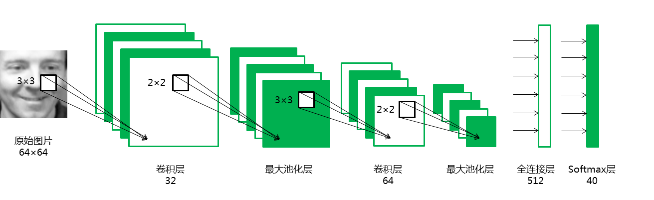
从keras的相应模块引入需要的对象:
from keras.models import Sequential
from keras.layers.core import Dense, Dropout, Activation, Flatten
from keras.layers import Conv2D, MaxPooling2D
from keras.optimizers import Adam
定义网络结构:
# 定义种子使参数初始化一致,从而实验可重复
seed = 100
np.random.seed(seed)

# 开始定义一个模型
model = Sequential()

# 添加一个卷积层,卷积核有32个,卷积核大小为(3,3),valid指卷积核只遍历有完整结构的数据
# input_shape最后一维为1代表输入是灰度图片,3代表彩色RGB图片
model.add(Conv2D(32, 3, 3, border_mode='valid', input_shape=(64, 64, 1)))
model.add(Activation('relu'))

# 添加池化窗口为(2,2)的最大池化层
model.add(MaxPooling2D(pool_size=(2, 2)))

# 添加一个卷积层,卷积核有64个,卷积核大小为(3,3)
model.add(Conv2D(64, 3, 3))
model.add(Activation('relu'))

# 添加池化窗口为(2,2)的最大池化层
model.add(MaxPooling2D(pool_size=(2, 2)))

# 添加Dropout层防止过拟
# Dropout将在训练过程中每次更新参数时随机断开一定比率的输入神经元
model.add(Dropout(0.25))

# 添加Flatten层把多维的输入一维化
# Flatten层常用在从卷积层到全连接层的过渡
model.add(Flatten())

# 添加有512个节点的全连接层
model.add(Dense(512))
model.add(Activation('tanh'))

# 添加softmax输出层
model.add(Dense(40))
model.add(Activation('softmax'))

# 定义损失函数与优化器
# 'categorical_crossentropy'用于多分类问题,优化器选择Adam
model.compile(loss='categorical_crossentropy', optimizer="Adam", metrics=['accuracy'])
3.4 模型训练与评估
用原始数据训练模型:
# 训练模型
model.fit(train_x, train_y, batch_size=200, nb_epoch=20, validation_data=(test_x,test_y))

# 模型评价
score = model.evaluate(test_x, test_y, batch_size=20)
print('Test loss:', score[0])
print('Test accuracy:', score[1])
更详细的模型评价:
pred=model.predict(test_x)
evaluate(pred,test_y)
用原始数据训练模型,能达到90%的准确率,其中错误较多的是把第17人识别为第22人、把第34人识别为第39人。
用增强后的数据训练模型:
需要注意:在重新训练模型之前,必须重新初始化模型参数,不然会从上次的训练结果开始迭代,导致出错。
# 训练模型
model.fit(train_x_enhance, train_y_enhance, batch_size=200, nb_epoch=20, validation_data=(test_x,test_y))

# 模型评价
score = model.evaluate(test_x, test_y, batch_size=20)
print('Test score:', score[0])
print('Test accuracy:', score[1])
更详细的模型评价:
pred=model.predict(test_x)
evaluate(pred,test_y)
同样的模型结构,增强数据能达到93.75%的准确率,即使识别错误,也最多错一次。
4 结果分析
两个模型的结果如下:
| model | loss | accuracy | precision | recall | f1-score |
|---|---|---|---|---|---|
| model_original | 0.571 | 0.900 | 0.93 | 0.90 | 0.90 |
| model_enhance | 0.291 | 0.938 | 0.94 | 0.94 | 0.93 |
画出柱状图直观展示两个模型的差异:
index=["loss","accuracy","precision","recall","f1-score"]
data=np.array([[0.571,0.291],[0.900,0.938],[0.93,0.94],[0.90,0.94],[0.90,0.93]])
df=pd.DataFrame(data,columns=["original","enhance"],index=index)
plt.figure(figsize=(8,6))
df.plot(kind="bar")
plt.ylim([0.2,1])
plt.show()

数据增强后的模型效果明显好于原始数据模型,这是因为训练数据的增多能降低过拟合,当遇到数据量较小的数据集时,应该优先考虑这种方法。