降维的主要作用包括减小计算量、去除数据噪音、有助于数据可视化等。PCA 是最常见的线性降维方法,常用的非线性降维算法包括自编码器和 t-SNE 等。本案例中,我们将使用 Python 实现 PCA 算法,使用实现的算法计算人脸数据集的特征脸。然后我们将使用 TensorFlow 构建自编码器,并应用于手写数字图像的重构。最后我们将使用一份中文新闻数据集,使用 Sklearn 实现的 t-SNE 算法对新闻进行降维,并使用 Seaborn 对降维结果进行可视化。
目录
- PCA 算法的 Python 实现
- 基于 PCA 的特征脸提取和人脸重构
2.1 加载 olivettifaces 人脸数据集
2.2 使用 PCA 对人脸进行降维和特征脸提取
2.3 基于特征脸和平均脸的人脸重构 - 使用 MNIST 手写数字数据集理解 PCA 主成分的含义
3.1 加载 MNIST 数据集
3.2 使用 PCA 对 MNIST 进行降维
3.3 基于手写数字可视化理解主成分含义
- 基于 AutoEncoder 的图像压缩与重构
4.1 使用 TensorFlow 构建自编码器
4.2 使用 TensorFlow 构建多层自编码器
- 中文新闻数据降维和可视化
5.1 新闻数据读取与向量化
5.2 使用 PCA 进行新闻降维和可视化
5.3 使用 t-SNE 进行新闻降维和可视化
- 总结
import numpy as np
def principal_component_analysis(X, l):
    X = X - np.mean(X, axis=0)#对原始数据进行中心化处理
    sigma = X.T.dot(X)/(len(X)-1) # 计算协方差矩阵
    a,w = np.linalg.eig(sigma) # 计算协方差矩阵的特征值和特征向量
    sorted_indx = np.argsort(-a) # 将特征向量按照特征值进行排序
    X_new = X.dot(w[:,sorted_indx[0:l]])#对数据进行降维
    return X_new,w[:,sorted_indx[0:l]],a[sorted_indx[0:l]] #返回降维后的数据、主成分、对应特征值
生成一份随机的二维数据集。为了直观查看降维效果,我们借助 make_regression 生成一份用于线性回归的数据集。将自变量和标签进行合并,组成一份二维数据集。同时对两个维度均进行归一化。
from sklearn import datasets
import matplotlib.pyplot as plt
%matplotlib inline
x, y = datasets.make_regression(n_samples=200,n_features=1,noise=10,bias=20,random_state=111)
x = (x - x.mean())/(x.max()-x.min())
y = (y - y.mean())/(y.max()-y.min())
fig, ax = plt.subplots(figsize=(6, 6)) #设置图片大小
ax.scatter(x,y,color="#E4007F",s=50,alpha=0.4)
plt.xlabel("$x_1$")
plt.ylabel("$x_2$")

使用 PCA 对数据集进行降维。
import pandas as pd
X = pd.DataFrame(x,columns=["x1"])
X["x2"] = y
X_new,w,a = principal_component_analysis(X,1)
将第一个主成分方向的直线绘制出来。直线的斜率为 w[1,0]/w[0,0]。将主成分方向在散点图中绘制出来。
import numpy as np
x1 = np.linspace(-.5, .5, 50)
x2 = (w[1,0]/w[0,0])*x1
fig, ax = plt.subplots(figsize=(6, 6)) #设置图片大小
X = pd.DataFrame(x,columns=["x1"])
X["x2"] = y
ax.scatter(X["x1"],X["x2"],color="#E4007F",s=50,alpha=0.4)
ax.plot(x1,x2,c="gray") # 画出第一主成分直线
plt.xlabel("$x_1$")
plt.ylabel("$x_2$")

我们还可以将降维后的数据集使用散点图进行绘制。
import numpy as np
fig, ax = plt.subplots(figsize=(6, 2)) #设置图片大小
ax.scatter(X_new,np.zeros_like(X_new),color="#E4007F",s=50,alpha=0.4)
plt.xlabel("First principal component")

Olivetti 人脸数据集。原始数据库可从(http://www.cl.cam.ac.uk/research/dtg/attarchive/facedatabase.html)。我们使用的是 Sklearn 提供的版本。该版本是纽约大学 Sam Roweis 的个人主页以 MATLAB 格式提供的。
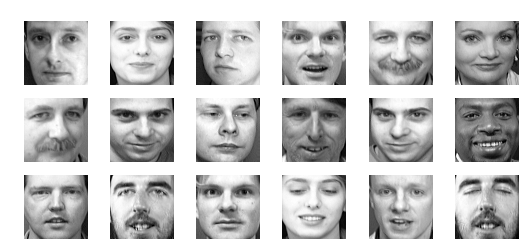
数据集包括40个不同的对象,每个对象都有10个不同的人脸图像。对于某些对象,图像是在不同的时间、光线、面部表情(睁眼/闭眼、微笑/不微笑)和面部细节(眼镜/不戴眼镜)下拍摄。所有的图像都是在一个深色均匀的背景下拍摄的,被摄者处于直立的正面位置(可能有细微面部移动)。原始数据集图像大小为 $92 \times 112$,而 Roweis 版本图像大小为 $64 \times 64$。
首先,我们使用 Sklearn 实现的方法读取人脸数据集。
from sklearn.datasets import fetch_olivetti_faces
faces = fetch_olivetti_faces()
faces.data.shape
选取部分人脸,使用 matshow 函数将其可视化。
rndperm = np.random.permutation(len(faces.data))
plt.gray()
fig = plt.figure(figsize=(9,4) )
for i in range(0,18):
    ax = fig.add_subplot(3,6,i+1 )
    ax.matshow(faces.data[rndperm[i],:].reshape((64,64)))
    plt.box(False) #去掉边框
    plt.axis("off")#不显示坐标轴
plt.show()

使用 PCA 将人脸数据降维到 20 维。其中 %time 是由 IPython 提供的魔法命令,能够打印出函数的执行时间。
%time faces_reduced,W,lambdas = principal_component_analysis(faces.data,20)
PCA 中得到的转换矩阵 $\mathbf{W}$ 是一个 $d \times l$ 矩阵。其中每一列称为一个主成分。在人脸数据集中,得到的 20 个主成分均为长度为 4096 的向量。我们可以将其形状转换成 $64 \times 64$,这样每一个主成分也可以看作是一张人脸图像,在图像分析领域,称为特征脸。使用 matshow 函数,将特征脸进行可视化如下。
fig = plt.figure( figsize=(18,4))
plt.gray()
for i in range(0,20):
    ax = fig.add_subplot(2,10,i+1 )
    ax.matshow(W[:,i].reshape((64,64)))
    plt.title("Face(" + str(i) + ")")
    plt.box(False) #去掉边框
    plt.axis("off")#不显示坐标轴
plt.show()

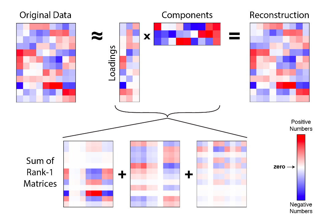
降维后数据每一个维度的作用,可以看做每一个主成分的权重。将原始图片的平均值加上不同主成分的权重和,可以对图像进行重构,如下图示例。
我们来随机选择一些人脸图片,观察一下图片的重构效果。
sample_indx = np.random.randint(0,len(faces.data)) #随机选择一个人脸的索引
#显示原始人脸
plt.matshow(faces.data[sample_indx].reshape((64,64)))

注意,由于 PCA 算法对图像进行了中心化,在重构人脸时还需要加上数据的平均值(这里称为平均脸)。
# 显示重构人脸
plt.matshow(faces.data.mean(axis=0).reshape((64,64)) + W.dot(faces_reduced[sample_indx]).reshape((64,64)))

对于每一个样本,降维后的每一个维度的取值代表的是对应主成分的权重。实际上就是利用不同特征脸的权重和再加上平均脸,才对原始人脸进行了重构。我们将上述样本的重构过程用图画出来。
fig = plt.figure( figsize=(20,4))
plt.gray()
ax = fig.add_subplot(2,11,1)
ax.matshow(faces.data.mean(axis=0).reshape((64,64))) #显示平均脸
for i in range(0,20):
    ax = fig.add_subplot(2,11,i+2 )
    ax.matshow(W[:,i].reshape((64,64)))
    plt.title( str(round(faces_reduced[sample_indx][i],2)) + "*Face(" + str(i) + ")")
    plt.box(False) #去掉边框
    plt.axis("off")#不显示坐标轴
plt.show()

3 使用 MNIST 手写数字数据集理解 PCA 主成分的含义
MNIST 手写数字数据集是在图像处理和深度学习领域一个著名的图像数据集。该数据集包含一份 60000 个图像样本的训练集和包含 10000 个图像样本的测试集。每一个样本是 $28 \times 28$ 的图像,每个图像有一个标签,标签取值为 0-9 。 MNIST 数据集下载地址为 http://yann.lecun.com/exdb/mnist/。
我们已经将数据集下载到 input/mnist.npz,可以直接读取。
import numpy as np
f = np.load("input/mnist.npz")
X_train, y_train, X_test, y_test = f['x_train'], f['y_train'],f['x_test'], f['y_test']
f.close()
将图像拉平成 784 维的向量表示,并对像素值进行归一化。
x_train = X_train.reshape((-1, 28*28)) / 255.0
x_test = X_test.reshape((-1, 28*28)) / 255.0
筛选出一个数字 8 的数据。
digit_number = x_train[y_train == 8]
随机选择部分数据进行可视化展示。
rndperm = np.random.permutation(len(digit_number))
%matplotlib inline
import matplotlib.pyplot as plt
plt.gray()
fig = plt.figure( figsize=(12,12) )
for i in range(0,100):
    ax = fig.add_subplot(10,10,i+1)
    ax.matshow(digit_number[rndperm[i]].reshape((28,28)))
    plt.box(False) #去掉边框
    plt.axis("off")#不显示坐标轴
plt.show()

利用我们实现的 PCA 算法函数 principal_component_analysis 将数字 8 的图片降维到二维。
number_reduced,number_w,number_a = principal_component_analysis(digit_number,2)
将降维后的二维数据集使用散点图进行可视化。
import warnings
warnings.filterwarnings('ignore') #该行代码的作用是隐藏警告信息
import matplotlib.pyplot as plt
%matplotlib inline
fig, ax = plt.subplots(figsize=(8, 8)) #设置图片大小
ax.scatter(number_reduced[:,0],number_reduced[:,1],color="#E4007F",s=20,alpha=0.4)
plt.xlabel("First Principal Component")
plt.ylabel("Second Principal Component")

我们首先提取降维之后的数据 number_reduced 的第一列数据 number_reduced[:,0],代表每一个样本在第一个主成分上的取值大小。按照取值从小到大进行排序,抽样提取原始的手写数字图片并进行可视化。
sorted_indx = np.argsort(number_reduced[:,0])
plt.gray()
fig = plt.figure( figsize=(12,12) )
for i in range(0,100):
    ax = fig.add_subplot(10,10,i+1)
    ax.matshow(digit_number[sorted_indx[i*50]].reshape((28,28)))
    plt.box(False) #去掉边框
    plt.axis("off")#不显示坐标轴
plt.show()

观察上图,可以看到数字 8 顺时针倾斜的角度不断加大。可见,第一个主成分的含义很可能代表的就是数字的倾斜角度。
同理,我们观察第二主成分的结果。
sorted_indx = np.argsort(number_reduced[:,1])
plt.gray()
fig = plt.figure( figsize=(12,12) )
for i in range(0,100):
    ax = fig.add_subplot(10,10,i+1)
    ax.matshow(digit_number[sorted_indx[i*50]].reshape((28,28)))
    plt.box(False) #去掉边框
    plt.axis("off")#不显示坐标轴
plt.show()

从 MNIST 手写数字训练集中采样一个图像子集,使用 Matplotlib 中的 matshow 方法将图像可视化。
rndperm = np.random.permutation(len(X_train))
%matplotlib inline
import matplotlib.pyplot as plt
plt.gray()
fig = plt.figure(figsize=(16,7))
for i in range(0,30):
    ax = fig.add_subplot(3,10,i+1, title='Label:' + str(y_train[rndperm[i]]) )
    ax.matshow(X_train[rndperm[i]])
    plt.box(False) #去掉边框
    plt.axis("off")#不显示坐标轴
plt.show()

TensorFlow 是谷歌公司著名的开源深度学习工具。我们借助改工具可以很方便地进行神经网络的构建和训练。自编码器是本质上是一种特殊结构的全连接神经网络。全连接层在 TensorFlow 中称为 Dense 层,可以通过 tensorflow.keras.layers.Dense 类进行定义。
首先,导入 TensorFlow 对应的模块。
import tensorflow as tf
import tensorflow.keras.layers as layers
在实际的神经网络训练中,可以使用 GPU 进行加速,在平台我们尚没有 GPU 资源,因此会默认使用 CPU 进行训练。
print(tf.test.is_gpu_available())
将图像拉平成 784 维的向量表示,并对像素值进行归一化。
x_train = X_train.reshape((-1, 28*28)) / 255.0
x_test = X_test.reshape((-1, 28*28)) / 255.0
构建一个自编码器,输入层大小为784,隐含层大小为 10, 输出层大小为 784 。在隐含层使用 ReLU 作为激活函数(非线性映射)。输出层则使用 Softmax 作为激活函数。自编码器模型构建步骤如下:
inputs = layers.Input(shape=(28*28,), name='inputs')
hidden = layers.Dense(10, activation='relu', name='hidden')(inputs)
outputs = layers.Dense(28*28, name='outputs')(hidden)
auto_encoder = tf.keras.Model(inputs,outputs)
auto_encoder.summary()
使用 compile 方法对模型进行编译。
auto_encoder.compile(optimizer='adam',loss='mean_squared_error') #定义误差和优化方法
使用 fit 在手写数字训练数据集上进行自编码器的训练。
%time auto_encoder.fit(x_train, x_train, batch_size=100, epochs=100,verbose=0) #模型训练
对训练集中的数据,使用自编码器进行预测,得到重建的图像。然后将重建的图像与原始图像进行对比。
x_train_pred = auto_encoder.predict(x_train)
# Plot the graph
plt.gray()
fig = plt.figure( figsize=(16,4) )
n_plot = 10
for i in range(n_plot):
    ax1 = fig.add_subplot(2,10,i+1, title='Label:' + str(y_train[rndperm[i]]) )
    ax1.matshow(X_train[rndperm[i]])
    ax2 = fig.add_subplot(2,10,i + n_plot + 1)
    ax2.matshow(x_train_pred[rndperm[i]].reshape((28,28)))
    ax1.get_xaxis().set_visible(False)
    ax1.get_yaxis().set_visible(False)
    ax2.get_xaxis().set_visible(False)
    ax2.get_yaxis().set_visible(False)
plt.show()

现在我们构建一个更深的多层自编码器,结构为 784->200->50->10->50->200->784。
inputs = layers.Input(shape=(28*28,), name='inputs')
hidden1 = layers.Dense(200, activation='relu', name='hidden1')(inputs)
hidden2 = layers.Dense(50, activation='relu', name='hidden2')(hidden1)
hidden3 = layers.Dense(10, activation='relu', name='hidden3')(hidden2)
hidden4 = layers.Dense(50, activation='relu', name='hidden4')(hidden3)
hidden5 = layers.Dense(200, activation='relu', name='hidden5')(hidden4)
outputs = layers.Dense(28*28, activation='softmax', name='outputs')(hidden5)
deep_auto_encoder = tf.keras.Model(inputs,outputs)
deep_auto_encoder.summary()
deep_auto_encoder.compile(optimizer='adam',loss='binary_crossentropy') #定义误差和优化方法
%time deep_auto_encoder.fit(x_train, x_train, batch_size=100, epochs=200,verbose=1) #模型训练
x_train_pred2 = deep_auto_encoder.predict(x_train)
# Plot the graph
plt.gray()
fig = plt.figure( figsize=(16,3) )
n_plot = 10
for i in range(n_plot):
    ax1 = fig.add_subplot(2,10,i+1, title='Label:' + str(y_train[rndperm[i]]) )
    ax1.matshow(X_train[rndperm[i]])
    ax3 = fig.add_subplot(2,10,i + n_plot + 1 )
    ax3.matshow(x_train_pred2[rndperm[i]].reshape((28,28)))
    ax1.get_xaxis().set_visible(False)
    ax1.get_yaxis().set_visible(False)
    ax3.get_xaxis().set_visible(False)
    ax3.get_yaxis().set_visible(False)
plt.show()

我们使用 Pandas 的 read_csv 方法将中文新闻语料读取进来, encoding 参数和 sep 参数分别设置为 "utf8" 和 "\t" 。使用 sklearn.feature_extraction.text 模块的 TfidfVectorizer,将词列表格式的新闻转换成向量形式。向量中的每一个维度代表字典中的一个词,维度的取值代表词在对应文档中的 TF-IDF 取值。
import pandas as pd
news = pd.read_csv("./input/chinese_news_cutted_train_utf8.csv",sep="\t",encoding="utf8")
#加载停用词
stop_words = []
file = open("./input/stopwords.txt")
for line in file:
    stop_words.append(line.strip())
file.close()

from sklearn.feature_extraction.text import TfidfVectorizer
vectorizer = TfidfVectorizer(stop_words=stop_words,min_df=0.01,max_df=0.5,max_features=500)
news_vectors = vectorizer.fit_transform(news["分词文章"])
news_df = pd.DataFrame(news_vectors.todense())
使用 PCA 将数据降维到二维。
from sklearn.decomposition import PCA
pca = PCA(n_components=2)
news_pca = pca.fit_transform(news_df)
将降维后的数据可视化出来。
import seaborn as sns
import matplotlib.pyplot as plt
plt.figure(figsize=(10,10))
sns.scatterplot(news_pca[:,0], news_pca[:,1],hue = news["分类"].values,alpha=0.5)

从上图可以看到,降维效果不是特别理想。不同主题的新闻在二维空间上互相重叠。下面我们使用 t-SNE 降维方法。
from sklearn.manifold import TSNE
pca10 = PCA(n_components=20)
news_pca10 = pca10.fit_transform(news_df)
tsne_news = TSNE(n_components=2, verbose=1)
%time tsne_news_results = tsne_news.fit_transform(news_pca10)
plt.figure(figsize=(10,10))
sns.scatterplot(tsne_news_results[:,0], tsne_news_results[:,1],hue = news["分类"].values,alpha=0.5)

可见,跟只使用 PCA 的方法相比, t-SNE 能够得到更好的低维新闻表示。
本案例我们首先使用 Numpy 实现了 PCA 算法,并应用于人脸数据集,对特征脸进行计算和可视化。然后,使用 TensorFlow 实现了自编码器和生层自编码器,在 MNIST 手写数字数据集进行训练。最后,在中文新闻数据集上应用 t-SNE 算法对新闻进行降维和可视化。
本案例使用的主要 Python 工具,版本和用途列举如下。如果在本地运行遇到问题,请检查是否是版本不一致导致。
| 工具包 | 版本 | 用途 |
|---|---|---|
| NumPy | 1.17.4 | 求解特征值和特征向量 |
| Pandas | 0.23.4 | 数据读取与预处理 |
| Matplotlib | 3.0.2 | 数据可视化 |
| Seaborn | 0.9.0 | 数据可视化 |
| Sklearn | 0.19.1 | 中文新闻的向量化、t-SNE降维 |
| TensorFlow | 1.12.0 | 自编码器的构建与训练 |