本案例借助TensorFlow构建对手写数字进行识别的多层感知机模型。
本案例主要包括以下内容:
1. 数据探索
2. 建立多层感知机模型
    2.1 创建对话
    2.2 定义相关函数
    2.3 设计网络结构
    2.4 定义损失函数与优化器
    2.5 模型训练
3. 使用Batch Normalization提升模型效果# 如果有CUDA
import os
os.environ['CUDA_VISIBLE_DEVICES'] = '3'
0 实验环境
import pandas, numpy, matplotlib, seaborn, sklearn, tensorflow
print "pandas:", pandas.__version__
print "numpy:", numpy.__version__
print "matplotlib:", matplotlib.__version__
print "seaborn:", seaborn.__version__
print "sklearn:", sklearn.__version__
tensorflow版本为0.12.1。
下面首先从tensorflow的examples中载入mnist数据集:
% config InlineBackend.figure_format='retina'
# 导入一些基础的包
import numpy as np
import pandas as pd

# 载入MNIST数据集
from tensorflow.examples.tutorials.mnist import input_data
mnist=input_data.read_data_sets("MNIST_data/",one_hot=True)
观察数据集结构组成:
mnist
观察发现,tensorflow中自带的mnist数据集被分为了三部分:train(训练集)、validation(验证集)、test(测试集),进一步观察数据集的结构与类型:
print "The shape of train set:", mnist.train.images.shape, mnist.train.labels.shape
print "The shape of validation set:", mnist.validation.images.shape, mnist.validation.labels.shape
print "The shape of test set:", mnist.test.images.shape, mnist.test.labels.shape
print "The data type of images:", type(mnist.train.images)
print "The data type of labels:", type(mnist.train.labels)
MNIST数据集被划分成了55000个训练样本、5000个验证样本和10000个测试样本,所有数据都以numpy数组形式存储,接下来我们需要在训练集上训练模型,在验证集上检验模型的效果并决定迭代何时终止,最终在测试集上评测模型效果。
下面我们进一步观察单个样本:
images原本是28×28的图片,但在tensorflow的mnist数据集中每张图片是以784维的向量形式存储的,展示图片时需要做维数变换,容易发现的是一维数组的存储方式放弃了图片的二维结构信息,一般情况下图片分类是不会这样的,但这个数据集的分类任务本身较为简单,所以简化了问题;labels有0-9共十个类别,以one-hot变量的形式存储;需要注意的是当用tensorflow处理多分类问题时,一般都使用one-hot形式的标签(可以使用tf.one_hot函数进行转换),因为目前多分类神经网络的输出层大多都是softmax层,该层的输出是一个概率分布,所以要求输入的标签也是概率分布的形式。
# 由于每张图片是以向量形式存储的,我们需要先将它转换为28×28的矩阵,才能展示图片。
number=np.random.randint(0,len(mnist.train.labels))
image=mnist.train.images[number]
image=image.reshape(28,28)

# 显示图片
import matplotlib.pyplot as plt
plt.imshow(image,cmap="Greys_r")
plt.axis("off")
plt.show()

# 输出其真实类别
arr=list(mnist.train.labels[number])
print "The real number in this picture is:", arr.index(max(arr))

2 建立多层感知机模型
2.1 创建对话
使用tensorflow需要先建立一个计算图,然后在与后端连接的session中运行它。一般而言,session可以通过tf.Session来创建,但是在交互式环境中(比如IPython和Jupyter),通过设置默认会话的方式更加方便,tensorflow提供了tf.InteractiveSession函数来自动生成默认对话。下面我们首先创建一个对话:
import tensorflow as tf
sess=tf.InteractiveSession()
2.2 定义相关函数
根据需要我们定义了两个函数:用于权重初始化的weight函数;用于评价模型效果的evaluate函数。
1)weight函数是为下一步设计MLP结构做准备的,Tensorflow中的参数初始值可以设置成随机数、常数或通过其他参数的初始值得到,通过满足正态分布的随机数来初始化weight是常用的方法,因为这样可以避免在使用RELU时出现完全对称或0梯度,bias的初始化一般选择常数。MLP因为是全连接网络,较其他神经网络的明显缺点是参数量大,容易过拟合,所以在设计模型时应该考虑一些防止过拟的技巧,比如在训练之前对数据进行增强、在初始化或定义损失函数时加入正则项、使用Dropout等方式。当网络结构复杂时,也可以定义初始化bias和选择激活函数的函数以简化结构。
2)evaluate函数是为了对模型效果进行评价的,其不仅可以输出分类问题的精度、召回率、F1值,还可以以可视化的方式观察混淆矩阵。
"""
函数weight(nodes_in, nodes_out, std, count)用来初始化权重
输入为:nodes_in(输入节点数)、nodes_out(输出节点数)、std(标准差)、count(衡量是否做正则化)
输出为:初始的weight
"""
def weight(nodes_in, nodes_out, std, count):
    w=tf.Variable(tf.truncated_normal([nodes_in,nodes_out],stddev=std))
    if count is not None:
        # 给weight做L2正则化处理,以控制参数量,防止过拟合
        weight_loss=tf.multiply(tf.nn.l2_loss(w),count,name="weight_loss")
        tf.add_to_collection("losses",weight_loss)
    return w

import seaborn as sns
from sklearn import metrics
from sklearn.metrics import classification_report

"""
函数evaluate(pred,testy)用来对分类结果进行评价;
输入:真实的分类、预测的分类结果
输出:分类的准确率、混淆矩阵等
"""
def evaluate(pred,testy):
    # 输出分类的准确率
    print("Accuracy: %.4f"  % (metrics.accuracy_score(testy,pred)))
    # 输出衡量分类效果的各项指标,包括精度、召回率、F1
    print(classification_report(testy, pred))
    # 更直观的,我们通过seaborn画出混淆矩阵
    %matplotlib inline
    plt.figure(figsize=(8,6))
    colorMetrics = metrics.confusion_matrix(testy,pred)
    # 坐标y代表testy,即真实的类别,坐标x代表估计出的类别pred
    sns.heatmap(colorMetrics,annot=True,fmt='d')
    sns.plt.show()
2.3 设计网络结构
下一步来设计MLP的基本结构,主要包括三部分:设置各个隐层的节点数、创建变量的placeholder、设计每层的结构。
1)输入层节点数就是特征images的维数,隐层的个数及其节点数的设计有很大的灵活性,一般根据数据集的复杂性和模型精度需要设计,理论上来说网络越深,越能挖掘到深层的数据关系。
2)tf.placeholder是用来存放数据的地方,第一个参数是数据类型,第二个参数代表tensor的shape,也就是数据的维度,所有需要输入模型的数据都需要放在这里,我们不仅需要定义输入、输出的placeholder,还需要定义模型中某些参数的placeholder,prob代表模型中Dropout的比率,Dropout是指随机将一部分节点置为0,而prob就是保存节点的比率,一般在训练时小于1,预测时等于1。
3)在设计每个隐层的结构时,最重要的是激活函数的选择,目前效果最好比较通用的激活函数是RELU,该函数与人类神经元的运作机制相似,能在一定程度上解决梯度弥散问题。另外在做二分类问题时,一般选择sigmoid(0、1)或者tanh(-1、1)作为最后一层的激活函数。
MLP模型的网络结构构建如下:
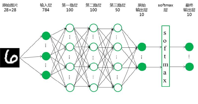
# 设置输入层节点数、隐层节点数
in_nodes=784
h1_nodes=100
h2_nodes=100
h3_nodes=50

# 定义输入、输出、prob的placeholder
x=tf.placeholder(tf.float32,[None,in_nodes])
y_=tf.placeholder(tf.float32,[None,10])
prob=tf.placeholder(tf.float32)

# 设置第一隐层
w1=weight(in_nodes, h1_nodes, 0.1, 0.005)
b1=tf.Variable(tf.zeros([h1_nodes]))
h1=tf.nn.relu(tf.matmul(x,w1)+b1)

# 设置第二隐层
w2=weight(h1_nodes, h2_nodes, 0.1, 0.0)
b2=tf.Variable(tf.zeros([h2_nodes]))
h2=tf.nn.relu(tf.matmul(h1,w2)+b2)
h2_drop=tf.nn.dropout(h2, prob)

# 设置第三隐层
w3=weight(h2_nodes, h3_nodes, 0.1, 0.0)
b3=tf.Variable(tf.zeros([h3_nodes]))
h3=tf.nn.relu(tf.matmul(h2_drop,w3)+b3)
h3_drop=tf.nn.dropout(h3, prob)

# 设置softmax输出层
w4=weight(h3_nodes, 10, 0.1, 0.0)
b4=tf.Variable(tf.zeros([10]))
y=tf.nn.softmax(tf.matmul(h3_drop,w4)+b4)
2.4 定义损失函数与优化器
对于多分类问题,通常都使用交叉信息熵cross_entropy作为损失函数,我们的目的就是不断训练使这个loss越来越小,直到到达一个全局最优或局部最优解。优化器我们选择有自适应学习率的AdaGrad,评价指标则是预测的准确率。
# 定义损失函数-交叉信息熵
cross_entropy=tf.reduce_mean(-tf.reduce_sum(y_*tf.log(y),reduction_indices=[1]))

# 选择自适应的优化器AdaGrad
train_step = tf.train.GradientDescentOptimizer(0.01).minimize(cross_entropy)
在训练模型之前,还需要做一点准备:定义计算准确率和用来维数转换的公式,tensorflow中的数据是以tensor(张量)类型存储的,与其他类型的数据并不兼容,所以若想要得到合理的可视化输出,我们一般先定义好tensorflow中的计算公式,之后再用eval函数将结果转换为numpy.ndarray等常见数据类型。
# 定义输出准确率的公式
# tf.argmax()函数用来输出一个tensor中最大值的标号,通过这个函数可以将one-hot型的类别变为标量型,再通过tf.equal()匹配预测正确的概率。
# 我们计算全部样本的预测准确度,先用tf.cast()将correct_prediction转变为float32,再做平均。
correct_prediction = tf.equal(tf.argmax(y, 1), tf.argmax(y_, 1))
accuracy = tf.reduce_mean(tf.cast(correct_prediction,tf.float32))

# 定义用来维数转换的公式
dimension_change1=tf.argmax(y, 1)
dimension_change2=tf.argmax(y_, 1)
2.5 模型训练
下面就可以开始训练模型了,next_batch函数可以每次都随机从训练集中抽取100个样本构成一个mini-batch,然后调用train_step对这些样本进行训练。
# 定义训练次数
# 定义列表存储相关指标
num_steps = 50000
test_acc = []

# 使用tensorflow的全局参数初始化器
tf.global_variables_initializer().run()

for step in range(num_steps):
    batch_xs,batch_ys=mnist.train.next_batch(100)
    train_step.run({x:batch_xs, y_:batch_ys, prob:0.75})

    if step % 50 is 0:
        acc_train=accuracy.eval({x: batch_xs, y_: batch_ys, prob:1.0})
        acc_valid=accuracy.eval({x: mnist.validation.images, y_: mnist.validation.labels, prob:1.0})
        acc_test=accuracy.eval({x: mnist.test.images, y_: mnist.test.labels, prob:1.0})
        test_acc.append(acc_test)
        pred=dimension_change1.eval({x: mnist.test.images, y_: mnist.test.labels, prob:1.0})
        testy=dimension_change2.eval({x: mnist.test.images, y_: mnist.test.labels, prob:1.0})
        acc=[step, acc_train, acc_valid]
        # 打印每一步的accuracy
        # print('Step # {}.  Train Acc :{:.4f}.  Valid Acc :{:.4f}  '.format(*acc))
print("Test accuracy: %.4f" % acc_test)
2.6 结果分析
下面输出更详细的效果评价:
print(evaluate(pred,testy))

观察发现,该模型对数字0、1的识别准确率较高,对数字9识别准确率相对较低;出现错误较多的是:把数字4和数字9混淆,把数字7错误识别为9,把数字3错误识别为5。
下面用图像来更直观地观察测试集上准确率的提升过程:
plt.figure(figsize=(8,6))
xx=np.array(range(0,len(test_acc)*50,50))
y1=np.array(test_acc)
plt.plot(xx,y1,"r-",label="MLP without BN")
plt.legend(loc="best")
plt.show()

可以发现,初期的收敛速度较快,后来趋于稳定,这可能是已经求得了全局最优解或局部最优解,如果使用SGD优化器,到这种时候可以调整为递进式学习率以跳出可能的局部最优解,但是AdaGrad本身就是自适应的学习率,不需再做这方面的调参。
3 使用Batch Normalization提升模型效果
Batch Normalization是一种重新参数化的策略,具体做法是在每一个mini-batch上进行Z-Score标准化,以此来减小层级传递中输出分布变化的不断放大。下面我们在原有的MLP模型基础上加上Batch Normalization,以观察其收敛速度的变化。
# 为BN操作准备的参数
epsilon = 1e-3

# 设置第一隐层
w1_BN = weight(in_nodes, h1_nodes, 0.1, 0.005)
z1_BN = tf.matmul(x,w1_BN)
batch_mean1, batch_var1 = tf.nn.moments(z1_BN,[0])
scale1 = tf.Variable(tf.ones([h1_nodes]))
b1_BN = tf.Variable(tf.zeros([h1_nodes]))
BN1 = tf.nn.batch_normalization(z1_BN,batch_mean1,batch_var1,b1_BN,scale1,epsilon)
BN1 = tf.nn.relu(BN1)

# 设置第二隐层
w2_BN = weight(h1_nodes, h2_nodes, 0.1, 0.0)
z2_BN = tf.matmul(BN1,w2_BN)
batch_mean2, batch_var2 = tf.nn.moments(z2_BN,[0])
scale2 = tf.Variable(tf.ones([h2_nodes]))
b2_BN = tf.Variable(tf.zeros([h2_nodes]))
BN2 = tf.nn.batch_normalization(z2_BN,batch_mean2,batch_var2,b2_BN,scale2,epsilon)
BN2 = tf.nn.relu(BN2)
BN2 = tf.nn.dropout(BN2, prob)

# 设置第三隐层
w3_BN = weight(h2_nodes, h3_nodes, 0.1, 0.0)
z3_BN = tf.matmul(BN2,w3_BN)
batch_mean3, batch_var3 = tf.nn.moments(z3_BN,[0])
scale3 = tf.Variable(tf.ones([h3_nodes]))
b3_BN = tf.Variable(tf.zeros([h3_nodes]))
BN3 = tf.nn.batch_normalization(z3_BN,batch_mean3,batch_var3,b3_BN,scale3,epsilon)
BN3 = tf.nn.relu(BN3)
BN3 = tf.nn.dropout(BN3, prob)

# 设置输出层
w4_BN = weight(h3_nodes, 10, 0.1, 0.0)
z4_BN = tf.matmul(BN3,w4_BN)
batch_mean4, batch_var4 = tf.nn.moments(z4_BN,[0])
scale4 = tf.Variable(tf.ones(10))
b4_BN = tf.Variable(tf.zeros(10))
BN4 = tf.nn.batch_normalization(z4_BN,batch_mean4,batch_var4,b4_BN,scale4,epsilon)
y_BN  = tf.nn.softmax(BN4)

# 定义损失函数-交叉信息熵
cross_entropy_BN=tf.reduce_mean(-tf.reduce_sum(y_*tf.log(y_BN),reduction_indices=[1]))

# 选择自适应的优化器AdaGrad
train_step_BN = tf.train.GradientDescentOptimizer(0.01).minimize(cross_entropy_BN)

# 定义输出准确率的公式
correct_prediction_BN = tf.equal(tf.argmax(y_BN, 1), tf.argmax(y_, 1))
accuracy_BN = tf.reduce_mean(tf.cast(correct_prediction_BN,tf.float32))
同时运行MLP without BN 和 MLP with BN,以此对比两种方法的收敛快慢。
# 定义训练次数
# 定义列表存储相关指标
num_steps=50000
accuracy_without=[]
accuracy_with=[]

# 使用tensorflow的全局参数初始化器
tf.global_variables_initializer().run()

for step in range(num_steps):
    batch_xs,batch_ys=mnist.train.next_batch(100)
    train_step.run({x:batch_xs,y_:batch_ys, prob:0.75})
    train_step_BN.run({x:batch_xs,y_:batch_ys, prob:0.75})
    if step % 50 is 0:
        acc_without=accuracy.eval({x: mnist.test.images, y_: mnist.test.labels, prob:1.0})
        accuracy_without.append(acc_without)
        acc_with=accuracy_BN.eval({x: mnist.test.images, y_: mnist.test.labels, prob:1.0})
        accuracy_with.append(acc_with)
        acc=[step, acc_without, acc_with]
        # 打印每一步的accuracy
        # print('Step # {}.  Accuracy without BN :{:.4f}.  Accuracy with BN :{:.4f}.  '.format(*acc))
print("Test accuracy without BN: %.4f Test accuracy with BN: %.4f" % (acc_without, acc_with))
下面用图像来展示两种方法的收敛过程:
plt.figure(figsize=(8,6))
xx=np.array(range(0,len(accuracy_without)*50,50))
y1=np.array(accuracy_without)
plt.plot(xx,y1,"r-",label="MLP without BN")
y2=np.array(accuracy_with)
plt.plot(xx,y2,"b-",label="MLP with BN")
plt.legend(loc="best")
plt.show()

由于数据前后的尺度差距较大,下面将其拆分为两段来观察:
fig=plt.figure(figsize=(20,7))
ax1=fig.add_subplot(1,2,1)
xx=np.array(range(0,len(accuracy_without[:100])*50,50))
y1=np.array(accuracy_without[:100])
plt.plot(xx,y1,"r-",label="MLP without BN")
y2=np.array(accuracy_with[:100])
plt.plot(xx,y2,"b-",label="MLP with BN")
plt.legend(loc="best")
ax2=fig.add_subplot(1,2,2)
xx=np.array(range(0,len(accuracy_without[100:])*50,50))
y1=np.array(accuracy_without[100:])
plt.plot(xx,y1,"r-",label="MLP without BN")
y2=np.array(accuracy_with[100:])
plt.plot(xx,y2,"b-",label="MLP with BN")
plt.legend(loc="best")
plt.show()

可以明显看到,加了Batch Normalization的MLP收敛的速度更快,以此验证了Batch Normalization对模型效果的优化功能。
4 小结
Yann LeCun教授整理的MNIST数据集是图像分类里最基础的数据集之一,近二十年来有很多研究者以此为训练集,研究图像分类领域的新方法。下面列举了几种模型在该数据集上的最好效果:
model=["KNN","Boost","SVM","MLP","CNN"]
best=[0.9948,0.9913,0.9944,0.9965,0.9977]
df=pd.DataFrame(best,columns=["best score"],index=model)
plt.figure(figsize=(8,6))
df.plot(kind="bar")
plt.ylim([0.99,1])
plt.show()

我们建立的MLP with BN可以达到0.9786的准确率,与效果最好的MLP模型还是有差距的,感兴趣的读者可以自己尝试去搭建上图中的MLP模型,该模型采用了六个隐层,节点数依次选择了:784、2500、2000、1500、1000、50,此类参数较多的模型对计算的要求较高,有条件的可以用GPU来训练。